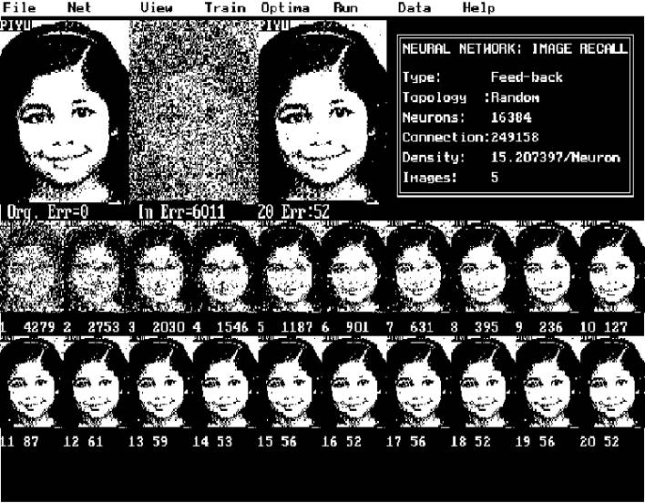
Figure (1) The input and output with randomly distributed noise.
| RENT A THINKER |
|
|
|||||
| Home | My Page | Chat | Tik-Tok | ||||
9.1
Abstract
9.2
Introduction
9.3
Network Topology
9.4
Training Algorithm
9.5
Results
9.6
References
Our brain has excellent associative image memory. We do not
understand it fully well as how brain stores and recalls images.
It is unlikely that natural neural circuits in our brain are fully and
orderly connected like Hopfield type network. Neurons are partially and randomly
interconnected in our brain. It is interesting to study the topology of such
networks and there properties. We will discuss about the techniques of building
partially randomly connected feedback type networks for associative memory
applications. We will also examine the methods of training and optimization of
such networks.
Hopfield type neural networks are used as
associative memory and for multi-variable optimization problems. In Hopfield
type network, generally binary output is used for each neuron. Generally the
output levels used are -1 or +1.
Inputs of every neuron are connected through network elements to all other
neurons' output through connections having appropriate weights. The input of a
neuron is computed by summing the of products of the output of all other neurons
and there corresponding connection weights to the given neuron as shown in
equation-1. The output of a neuron is updated using equation-2, by hard clipping
the sum of input values. Generally the output is +1 or -1 depending on the sign
of the input. To store a set of patterns in these network the connection weights
are fixed using Hebb’s rule [equation (3)].
Hopfield's network-
N-1
Yj(t+1) = fnå [ Wij * Yi(t) ]
for (i <> j) .......(1)
i=0
fn[x] = -1
for x < 0
=
1 for
x >= 0
.......(2)
Where Yj(t+1) is updated state of the neuron,
Yi(t) is earlier state of the
neuron,
Wij is the connection strength
between
output of Yi
and input of Yj,
N is the total number of neurons.
Assigning of weights-
M-1
Wij = å Yi(s)*Yj(s)
.......(3)
0
where i <> j,
Wij is the connection strength between
input of Yj and output of Yi,
M is number of patterns and,
for i=j, Wij=o.
These networks exhibit the property
of recalling the originally trained image from a partial or a noisy input
pattern. The interconnection requirements for such a fully connected network is
[ N ( N - 1) ], where N is the number of neurons in the network.
A Hopfield type neural network is often used for imaging applications, in
which each neuron represents a pixel. However in Hopfield model, number of
interconnections increases exponentially with increases of neurons.
Number of interconnections required for a picture having 128 X 128 (16K)
pixels is approximately 250 million. The time taken to compute the stable state
of the network output is very high for any practical application. The number of
patterns that could be stored in a Hopfield type network is approximately 0.15
times the total number of neurons in the network Brain has excellent associative image
memory and yet we do not understand fully well the mechanism of storing and
recalling used by the brain.
It is unlikely that natural neural circuit in our brain is fully and
orderly connected like Hopfield network. It is connected randomly with a
constrain of geometric weighting function deciding the interconnection density.
Connection probabilities with neighboring neurons are higher than the ones at a
distance.
The work done in this area is at a very
primitive stage. One of the reasons for this is the high computational
requirement. Even to experiment with a low quality binary image we need very
large memory and CPU time.
In view of the above a randomly connected
feedback type network model is developed using limited interconnections. Using
this method a factor of thousand memory saving is possible with equivalent
increase in speed . A prototype network is designed for 128X128 binary picture
containing N=16K neurons. Each neuron input has only few (C = 7 to 40) network
elements connected to the outputs of randomly selected neurons. 250 thousand
interconnections are used instead of 250 million connections required for fully
connected network. This gives an advantage
of 3 orders of magnitude in
computation time and memory requirement. By connecting these elements
homogeneously but randomly between the neurons, we have [ (100 X C)/N % ] 0.1%
probability (for C=16) of any two neurons being
connected in a positive feedback loop. To increase this probability
various random network topologies are developed for different types of noise present in the recall pattern. The Hebb's rule was found
inadequate for optimally storing the images in above type of network. An
iterative training strategy is developed that converges the output error to less
than 0.01% to 0.1%. For efficient computation, a topological mapping function is
generated for each connecting element. The network topology is defined in a
separate mapping file, which is used, for computation of 'recalls' and
'training' algorithms. A network of size 128 x 128 neurons and 7 links
per neurons is used to train seven binary images. Interconnection weights are
first computed and then adopted by applying iterative correction proportional to
the output error. After the training, the network is tested with any one of the
seriously degraded, rotated or shifted images.
Putting random value to randomly chosen pixels or continuous cluster of
pixels performs the pixel degradation. Alternately the input image is rotated by
a small angle or shifted in both x and y coordinates before presenting to the
network (see fig-2).
One of the network topologies developed
that gave optimal performance is designed to divide the association into two
groups (I) for near and (II) for
far neurons. Part of the interconnections is distributed to adjacent neurons and
the other part of the interconnections is distributed over the rest of the
neurons. While doing this the probability of positive feedback (i.e. two neurons
connected back to back) is increased using external constrain.
To optimize the training time the network elements are computed using Hebb's rule [equation (3)]. A bias link is added to each neuron that is found to reduce the error in iterative training mode. The network is trained by computing the analog error with respect to a dynamic threshold value. The link weight correction is applied proportional to the analog error. Figure (2) shows the error convergence curve with and without Hebbian rule applied.
Table (1) Number of images
successfully recalled v/s number of elements per neuron.
Figure (1) The input and
output with randomly distributed noise.
Figure (3) Rotted image
response.
[1] Lippmann R.P.,
An introduction to computing with Neural Nets. IEEE ASSP Magazine, pp
4-22, 1987.
[2] Griff Bilbro etal, Optimization
by Mean Field Annealing Advances in Neural Information Processing Systems I.
[3] Robert J. Marks II etal,
Alternting Projection Neural Networks. IEEE transations on circuits and systems,
Vol. 36, No. 6, JUNE 1989.
[4] Nikitas J. Dimopoulos, A Study
of the Asympotic Behavior of Neural Networks. IEEE transations on circuits and
systems, Vol. 36, No. 5, MAY 1989.