7
A
Neural Network Tool Box using C++
7.1
Abstract
7.2
Introduction
7.3
On Tool Box Implementation
7.3.1
Neural Net Designer-1 (For Feed Forward Type Network)
7.3.2
Neural Net Designer-2 (For Feed Back Type Network)
7.3.3
Neural Net Designer-3 (For Unsupervised Learning)
7.4
Proposed Algorithm for Pruning
7.5
Results
7.6
Conclusion
7.7 References
6.14
PUBLISHED
An interactive Neural Network developing Tool Box is designed using C++.
The Neural Networks are emerging computational technique used for artificial
intelligence applications. Neural Networks are used for speech and image
recognition, feature extraction, and associative memory applications. For
simulation of Neural Network OOPs (Object Oriented Programming) are found most
suitable programming language. The paper describes in general the Neural Network
optimizing algorithms used in above implementation illustrated with results.
Artificial Neural Network (ANN) is a problem solving
technique, which tends to simulate the natural system of brain. ANN is in far
too primitive stage compared to the brain of lowest biological species. This is
mostly because of the complexities of the biological systems. ANNs are
inherently parallel processing technique. Increase of processing power is almost
proportional to the number of processing elements in an ANN system. There are
two important characteristics of ANN systems:
- Similar processing is performed in large number
of data sets.
- Different operations are performed on same data
set.
In multilayer type network, there
are similarities of the data structures of different layers. Also there are
different processes like network updating, network weight reinforcement, network
monitoring, network loading and network saving etc. which work on same data set.
These two properties of ANN are also the important properties of object oriented
programming languages. Data hiding is another important aspect of OOP, which is
relevant to ANN implementation. In ANN the certain data structures are
associated with specific operations only. For example, the delay time of delay
neurons or the address map of random interconnections are processed by certain
objects or friendly objects only. OOP hides the complexities of data structure
from the higher-level programming. Considering the features of OOP and ANN, a
general-purpose toolbox is designed using Borland C++.
This toolbox consists of three
packages. These packages are: “Neural Net Designer Part I, II and III for Feed
Forward type multi layer networks, feedback type networks and for self learning
type neural networks respectively”. Brief overview of these packages with the
details of the aspects like network configuration and network optimization is
given below.
The packages are designed in three parts. In all the
packages, a self contained integrated environment is created based on
interactive window to develop Neural Network type applications with online
graphics display. The systems have following main features. The packages are
dedicated for Feed Forward, Feed Back, and Unsupervised learning.
·
Interactive and user friendly window
·
Real time graphics display
·
Network view
·
User definable and standard neuron activation functions and
summing functions
·
Flexible connectivity, layered and random connections
·
Learning and forgetting coefficients
·
Optimizing of network
·
Graphics and numeric data generation support
·
Run time probing of neurons
·
Time series prediction using delay neurons
·
Image band compression using feature extraction
·
Interactive and user friendly window
·
16K neurons and 1 million connections
·
0.1 million connections per second while using 486 based PC.
·
Maximum image size (128x128)
·
Random connectivity
·
Auto network building with optimized connections
·
Recall with noisy, offsetted and tilted images
·
Recall response 2.5 sec. in 486 based PC
·
Data generation and import of images from other files
·
Interactive and user friendly window
·
Supports most features of Multi Layered NN
·
Mixed mode operations for supervised and unsupervised
learning
·
Network view
·
Probing of hidden neuron outputs
·
Data generation
Feed Forward type multilayered Neural Networks are very
popular for their generalization and feature extraction property. However the
Feed Forward type network need supervised learning to train the network
initially. Self-organizing networks on the other hand are used in application of
image classification, speech recognition, language translation, etc. An
algorithm is developed to train multilayered Feed Forward type network in both
supervised and unsupervised mode. Unsupervised learning is achieved by enhancing
the maximum output and de clustering the crowded classes simultaneously.
Proposed algorithm allows to force any output to learn a desired class using
supervised training like Back Propagation. The network uses multilayered
architecture and hence it classifies the features. Population of each class
could be controlled with greater flexibility.
There are various new concepts incorporated in the “Neural
Net Designer” systems. There are capabilities of random connectivity, time
delay neurons, use of complex neuron activation function etc. Among these the
most useful feature of the system is network pruning. The following section
describes the pruning algorithm used in our system.
Configuration of optimal network for an input and output data
set depends on the type of neurons selected in hidden layer. We still do not
have a method to select appropriate type of neuron for a problem. However, the
algorithm optimizes the network by selecting most appropriate type of neurons
available in the network and their interconnections. Following are different
steps of the optimization.
Step
1:
Choose a multilayered network, which is already trained with desired
input output data sets and has output error well below the desired value Emax.
Step
2:
Train the net, for a single pass with complete training using back
propagation algorithm.
Step
3:
Reduce magnitude of all connections using Wij = Wij * nf where nf is
forgetting coefficient, less than but close to 1.0.
Step
4:
Repeat the step 2 and 3 till total error minimizes well below desired
limit Emax.
Step
5:
use successive approximation method as shown in the flow chart of figure
4 to remove the connection till error is > Emax. Sort the connections for
every pass when the connections are removed.
Step
6:
Remove all neuron with no input connection or no output connections.
Step
7:
Neurons having single input or single output are removed and connections
are reorganized appropriately.
Step
8:
If step 7 is applicable then train the network again.
The above algorithm is tested with a fully connected
multilayer neural network having more than one independent input-output
function. For example we consider a network having inputs A, B, C, D and outputs
P and Q such that P = A xor B and Q = C xor D.
To solve given problem, a fully connected network is
configured with four hidden neurons h1, h2, h3, and h4. After optimization the
networks corresponding P and Q are isolated from each other. Also two hidden
neurons h3 and h4 are eliminated (see fig – 5). In the second case, a
two-dimensional image-mapping problem is examined. A network is configured
initially with two analog inputs, thirteen hidden neurons in a single layer and
an output neuron with binary output. Twelve hidden neurons input are of the form
–
Xj = ∑ (Wij * Yi) and
Yj = 1 / (1 + ex) …..(1)
Only one hidden neuron input is used with special summing
function –
Xj = ∑i (Wij * Yi2)
and Yj = 1 / (1 + ex)…….(2)
The network is trained to map a circle and then the network
is optimized using above technique. Optimization result is shown in figure 6.
The resultant network has only one hidden neuron and three connections. The
neuron ‘selected’ by the optimization is the one, which is specially
implanted in the network to solve the problem of circular boundary. Each of the
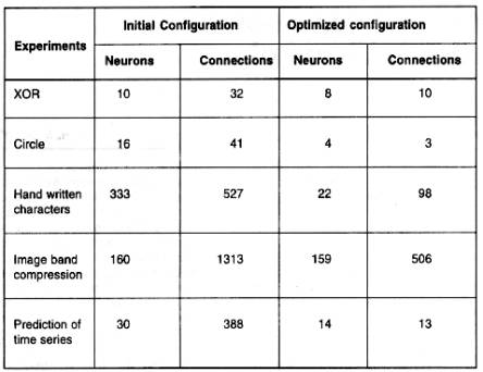
above experiment is conducted ten times, and the results are shown in table 1.
The above optimization algorithm is used in several other applications like (a)
mapping of handwritten characters, (b) prediction of time series functions (c)
complex Boolean functions and (d) image band compression etc.
Optimization of multi layer neural network is achieved by
removing weakest connections from the network. Optimization of network has
following advantages.
1.
Reduces network size to minimum by optimizing the use of
neurons and connections.
2.
Possibility of VLSI design
3.
Isolation of independent variable
4.
Easy to realize internal representation.
Using above technique it is possible to design run time
auto configuration of the network topology.
1.
Lippman R. P., An introduction to computing with neural nets.
IEEE ASSP Magazine pp 4-22, April 1987.
2.
D.E. Rumalhert and J.L. McClelland, Parallel Distributed
Processing Explorations in the Micro structure of cognition. Cambridge MA:MIT
press, vol 1, 1986.
3.
R. Hetcht-Nielsen, “Theory of the back propagation neural
network”, In Proc. Int. Joint. Conf. Neural Networks, vol 1. pp-593-611. New
York: IEEE press, June 1989.
4.
E. D. Karnin “A Simple procedure for pruning back
propagation trained neural network”, IEEE Trans, Neural Networks Vol. 1, pp
239-244, June 1990.
|
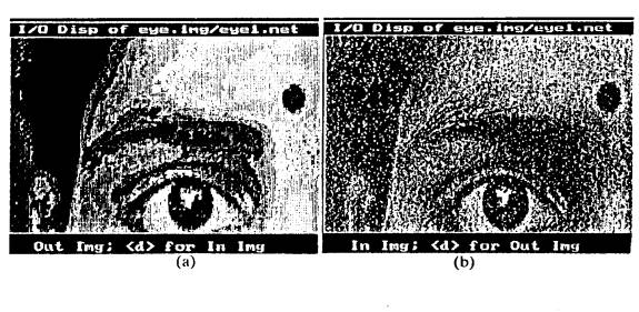
Fig 1 – Image band compression using 64-12-8-64
FFNN with 8x8 image window.
(a) is the output image corresponding to (b) 256x256x16 noisy gray image.
|
|
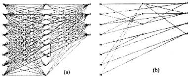
Fig
2 – Network optimization using “Neural Network Tool Box –1”.
Figure (a) & (b) are FFNN to solve XOR problem before and after
optimization respectively.
|
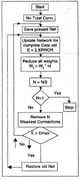
Fig 4 – Network Optimizing Algorithm, where Emax is the maximum
tolerable error.
|
|
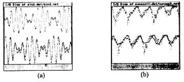
Fig
3- Time series prediction using Delay neuron in FFNN. (a) Complex
periodic waveform (top trace) is predicted (bottom traces) along with
expected output. (b) Shows 55 years sunspot activity by time delay FFNN.
|
|
Figure 5 – Configuration of network before and
after optimization. The above network is trained for P = A xor B and Q = C
xor D. Optimized network on the right has split in two parts isolating two
independent problems P and Q.
|
|
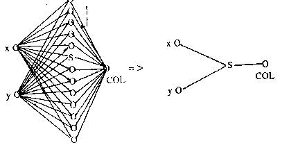
Fig 6 – In above example let R = ((X + 0.5) 2
+ (Y - 0.5) 2) 0.5 and if (R < 0.3) then
COL = 0 else COL = 1. X and Y are random analog inputs between 0 and 1. A
special neuron S (See text) is implanted among the hidden neurons. In the
network on the left. On the right is the optimized network where all the
hidden neurons are replaced by a single special neuron S.
|
|
|
Table
1 – Results of network optimization for different types of input
outputs. Optimized configuration presented here are average of ten
experiments each started with different initial weights.
|
|
|
|
7.8 Published
Himanshu S. Mazumdar
& Leena P. Rawal, "A
Neural Network Tool Box using C++", in CSI Communications, April, pp.
22-25, Bombay, 1995. Himanshu S. Mazumdar &
Leena P. Rawal, "A Neural
Network Tool Box using C++ ", in CSI Communications, August, pp. 15-23,
Bombay, 1995.(This paper has received "Best Article of the Month
Award")