| RENT A THINKER |
|
|
|||||
| Home | My Page | Chat | Tik-Tok | ||||
6.1
ABSTRACT
6.2
INTRODUCTION
6.3
STOCHASTIC TYPE MULTI- LAYER ARTIFICIAL NEURAL NETWORK
6.4
Proposed algorithm
6.5
CHOICE OF HIGHER FUNCTIONAL BLOCKS
6.6
Pre-trained MLP (Multi-Layer Perceptrons) block
6.7
Look up table
6.8
Time delay neuron
6.9
Functional neuron
6.10
PRUNING ALGORITHM
6.11
RESULTS
6.12
CONCLUSION
6.13
REFERENCES
6.14
PUBLISHED
A large
randomly connected Feed Forward type Neural Network (FFNN) is designed to solve
a class of problems. This network is used to test and simulate the possibility
of hybrid of FFNN and other types of computing elements. The higher functions
building blocks are simulated as artificial neurons and are implanted in the
above network. The composite network is trained and pruned. As a result, it is
observed that, the original network adopts the implanted building blocks and the
total size of the network reduces considerably. The suitable reverse
characteristics of each functional block are designed to implement training
using gradient descendent technique. Some of the building blocks are designed
using stochastic type logic. Such building block’s output is similar to the
output of the biological neuron. This work is carried out in the view of future
possibility of bio-electronic (hybrid) systems.
The objective of our work is to demonstrate the possibility
of implantation of non-neural computing devices in the simulated randomly
connected Artificial Neural Network (ANN). To test the above possibility, a
large randomly connected feed forward type host ANN is designed using a
general-purpose neural network tool box [6].
Small independent functional building blocks are designed to simulate artificial
neurons. Some of the hidden neurons of the host network is chosen at random and
is replaced with above functional blocks. The host network is then trained to
solve a specified problem using supervisory learning algorithm. The composite
network is then pruned [2][3] to
optimize the size of the network. The resultant network is a reduced size hybrid
of neural and other type of building blocks. It is observed that the implanted
functional blocks that were most appropriate to the problem, were adopted by the
host network. Such hybrid system
allows computer simulation of large ANN architecture with faster response time.
There are three main designing aspects of the above type of network as described
below -
·
the stochastic type ANN design,
·
choice of higher function building blocks
and
·
pruning algorithm to optimize the network size.
The following section describes the above aspects in detail.
The section II of this paper describes the stochastic [1] learning algorithm developed for VLSI implementation [5].
The algorithm is similar to the Back Propagation algorithm but can use binary
neurons at hidden nodes. Such neuron’s outputs is probabilistic in nature and resembles output of biological neuron. Section III describes
the different types of higher functional building blocks. Using these functional
blocks, different applications are developed. Some of the results are given in
section V. The Section IV describes the pruning algorithm. An iterative pruning
algorithm is developed, which optimizes the network size. In many examples like
XOR, circle mapping etc., this algorithm optimizes the network size to the
theoretical minimum limit. The section V describes the results of different
experiments conducted as mentioned in section II, III and IV. Finally, section
VI gives conclusion and useful references are listed at the end.
We first review briefly the back propagation (BP)
technique [7] that is popularly used for training FFNNs. The input-output
characteristic function (activation function) of a neuron is chosen such that it
is continuous and its first derivative is bounded between definite limits for
large dynamic range of input. Consider a three layer network of units Yi,
Yj and Yk which are interconnected through weights wji
and wkj such that-
Xj =
åi
wji * Yi;
Yj
= f(Xj); (second layer)
Xk
= åj
wkj * Yj;
Yk
= f(Xk); (third layer)
Here Y = f(X)
represents the neuron activation function of the form f(X) = 1/(1+e(-X)).
The weights wkj
and wji are modified using
the BP algorithm as follows-
wkj = wkj
+ h
* Yj * (Yk-dk)
* {Yk * (1-Yk)}
....(1)
wji = wji
+ h
*Yi *{Yj
*(1-Yj)} * Sk
[(Yk-dk)*{Yk
*(1-Yk)}* wkj]
....(2)
where h is a real
constant less than 1.0 and dk
is the desired output. Theoretically, a three-layer network is sufficient for
mapping any given input-output set. For reasons of efficiency, however, it may
be necessary to consider networks with more than 3 layers. It is straightforward
to modify the above equations for the applications having more than 3 layers.
All the variables except
Yi
and dk
of equation (1) and (2) are real
variables and hence difficult to implement in VLSI for parallel processing of a
large number of perceptrons. It has been shown that the choice of perceptron’s
characteristic [4] is not very
critical for convergence of error during training. This paper suggests one such
choice that reduces the computational requirement drastically without effecting
the error convergence property during training.
We will analyze the significance of each factor in expressions
(1) and (2) in order to
replace them by suitable probability functions-
[Yk-dk]
is the departure of output Yk
from the desired value dk.
[Yk
* (1-Yk)]
is the measure of willingness of Kth output neuron to learn. This is
measured by its nearness from its average value (0.5). This factor plays an
important role in training.
[wkj
]
is the back propagation
signal path’s conductance.
[Yj
* (1-Yj)] is similar to the
above term {Yk * (1-Yk
)} for hidden layer neuron
[Yi] is the excitation potential for ‘wji’.
In the proposed system the perceptron’s forward pass
transfer characteristic is generated by a threshold detector having a random
bias value as shown in figure-1.
This is equivalent to a choice of input-output characteristic function of
equation (3).
Y = 1 for (X + r) > 0; and
Y = 0 for (X + r) <= 0 ;
...(3)
Here r is a random
integer inside the dynamic range of Xj.
Yj and Yk
are calculated using the above equation
-(3) in the forward pass. This has two advantages: the value of Yj
is binary but is statistically continuous in the dynamic range of learning and
the computations of Xk
(for the next layer) does not need any multiplication.
In the backward pass, a term of the form Yk
* (1-Yk) is desirable. This term increases the sensitivity of wkj
near the threshold value of Xk.
Equivalently, the network’s willingness to learn or forget is inversely
proportional to the distance of Xj from the threshold. Considering this, a
simplified reverse characteristic function R(X),
as shown in figure-1 and equation (4),
is used to replace the terms of the form {Y
* (1-Y)} in equations (1) and (2).
R(X) = 0 for abs(X) > r; and R(x) = 1 for
abs(X) <= r;
...(4)
Here r is a
positive random integer less than N and
the dynamic range of the X for
learning is
-N
to +N . The value of N is
dependent on the network configuration. To improve the dynamic range of the
X’s and the rate of convergence, one of the following methods is used -
·
Use
N as random integer;
·
Use
‘r’ as weighted random number;
·
Adjust
the value of N gradually as error converges.
| Curve-1 (dotted line) p=N-random(2*N+1)+X if p>0 then z=1 else z=0 Y=(Ss zs)/S for S samples Curve-1 (solid line) Y = 1 / 1+ e(-X) |
Curve-2 (dotted line) p=random(N)-abs(X), f p>0 then z=1 else z=0 y=(Ss zs )/S for S samples Curve-2 (solid line) Y= e(-X) /(1+ e(-X)) 2 |
Figure - 1 The forward and the
reverse characteristics of the proposed stochastic function
along with exponential
sigmiod function in solid line.
The error convergence curve of a simple 3 layer stochastic
type network is shown in figure-2,
using XOR input-output function. Figure-3(a)
and 3(b) show the output of some of the stochastic type hidden neurons in
time domain and the output of a biological neuron respectively. The figure shows
the similarity between the stochastic and biological neuron.
Different types of special type of neuron functions are
developed to increase the efficiency of training in a complex network
environment. Each of such functional blocks is equivalent to several artificial
neurons and associated connections of conventional neural circuit. The
functional blocks are implemented using dedicated hardware or micro-processor
based system. A general purpose Neural
Network Tool Box [6]
is designed to interface different types of functional building blocks with
multi-layered FFNN. The Tool Box is a computer simulation program, which
supports interactive design of network topology, new activation function and
training algorithm. Some of the functions developed using above Tool Box are
described below-
To reduce the training time, it is
convenient to train separate functional blocks of multi-layer FFNN. These
functions are generic in nature like image band compression, time series
prediction, geometric mapping functions for circle, ellipse, polygon etc.. The
pre-trained blocks transfer the BP error like normal FFNN. The elements of these
blocks are not reinforced during training.
To simulate above type of pre-trained network block, the Neural
Network Tool Box is used. A portion of a large network is first trained
using XOR problem. Then the selected weights
are inhibited to reinforce the values during training. The composite
network is trained with a function, that uses XOR operation- e.g.
(AÅB) OR (cÅD). The figure-
7(a) and 7(b) show the network,
before and after pruning, respectively.
Figure - 2
The error convergence curve of a 3 layer stochastic type Feed Forward
Neural Network.
Figure- 3
Similarity between the stochastic and the biological neurons. (a) Output of
stochastic type neurons (see
text). The curves h1, h2, h3
& h4
are hidden neuron’s output
during training
for fixed
input pattern.
The X-axis
represents iteration (@
10 samples per iteration). (b)
Output of biological neurons..
For binary input-output operation, boolean functions and look
up tables are used, which are integrated with a host network using stochastic
learning algorithm. This gives higher flexibility, density and speed.
Appropriate reverse characteristics are designed using stochastic type
functions.
For efficient representation of the time domain signal, time
delay neuron is introduced. The time delay neuron retains history of time series
input signals in the hidden neurons of the
network. A time delay neuron receives the input from the immediate neighboring
neuron, retains the value for ‘d’
period of integer delay and outputs like normal neuron. These neurons allow
variable unit of integer time delay as shown in the equation (5).
Yj(t) = Xj(t-dj)
...(5)
where ‘dj’
is the integer time delay of j th
delay-neuron and ‘t’
is the time.
Figure
- 4 The organization of the time
delay neuron.
![]() The
total time delay Td of all
the neurons in a
time delay
network is given by - Td=Sj
dj.
Figure-4 shows the organization
of time delay neurons as a functional building block. There is a single input
Yi, which is delayed through different delay neurons
Yj. The output of delay neurons Yj
s are connected to Yks, the output neurons. The above building block retains the
time domain information in Yj
neurons. Using such building blocks, it is possible to generate functions of the
convolution of input signal, standard filters, time series prediction etc.. One
of such applications shown in figure-5
is time series prediction. The network of figure-4
is trained to predict a complex time series function.
The
total time delay Td of all
the neurons in a
time delay
network is given by - Td=Sj
dj.
Figure-4 shows the organization
of time delay neurons as a functional building block. There is a single input
Yi, which is delayed through different delay neurons
Yj. The output of delay neurons Yj
s are connected to Yks, the output neurons. The above building block retains the
time domain information in Yj
neurons. Using such building blocks, it is possible to generate functions of the
convolution of input signal, standard filters, time series prediction etc.. One
of such applications shown in figure-5
is time series prediction. The network of figure-4
is trained to predict a complex time series function.
Functional neuron is a neuron that is pre-defined function
(equation) which may be equivalent to several neurons and interconnections. One
of the trigonometric and algebraic functions are studied are given in equation
(6).
Xj
= ( åi
(W * Yi 2) ) 0.5
;
...(6)
The use of functional neuron drastically reduces the network
size and increases the speed of operation. These types of neurons are
appropriate for real time applications for modeling, image prediction, pattern
recognition etc. Use of functional neurons also facilitates in building
mathematical model from the observed data. This is achieved by studying the
topology and inter-relationship of
functional neurons inside the network. Section-V describes the results of
circular boundary mapping using the neuron activation function of
equation (6).
The
method described above are integrated with a host network. For each method
suitable error propagation strategy is developed, to reinforce the components of
the host network. In case of the functions, which are not differentiable, the
stochastic method as described in section II, is used. The composite network is
simplified using pruning algorithm as described in section below.
A
simple but efficient technique is developed which reduces the size of the
network almost to the theoretical limit with minimum number of trials. The
method is based on the simple fact that in a trained network, useful connections
are stronger and the unwanted connections are weaker. The effect is further
enhanced by slowly reducing the strength of all the interconnections with time.
The operation is
analogous to
forgetting. When
learning and
forgetting reaches
equilibrium,
Figure
- 5 (a) A fully connected FFNN configuration with a time-delay
functional block trained for time series prediction.
(b) The resultant network after training and pruning.
(c) & (d) The input signal (top trace) and the predicted
output(bottom trace) of the network (a) & (b).
the optimum configuration connections are stabilized. When
equilibrium is reached, the weakest connections are gradually eliminated using
successive approximation method, until the network’s output error is less than
or equal to a desired error limit. As a result of the reduced connections, some
neurons will have no input or will have only single input-output connection.
These neurons are eliminated by using appropriate rules and connections are
rerouted. The figure-6 shows the
Flow-chart of the pruning algorithm. The figure-5,
7, 8 and 9 shows the result of pruning in different applications.
Using the above techniques, several experiments were
conducted to test the feasibility of implanting non-neural functional blocks, to
a redundantly connected large host FFNNs. In most cases, it was observed that,
the host network adopts the implanted functional blocks. The implanted
functional blocks participate in solving problems and a large portion of the
other network elements becomes redundant. Hence, the network size minimizes
considerably after pruning. Some of
the cases studied are given below-
Experiment - I :
XOR problem
A fully connected multi-layer FFNN is configured using two
pre-trained network h1, h2. h5, P and
h3, h4, h6, Q. The network has four inputs a, b, c, d and one
output R, as
shown in
the figure-7(a). The network is trained and pruned as explained in
section-IV using the function -
R = (AÅ
B) OR (CÅ D).
After
pruning, the networks corresponding to P and Q are automatically isolated from
each other. Also the four redundant hidden neurons are eliminated as shown in figure
7(b).
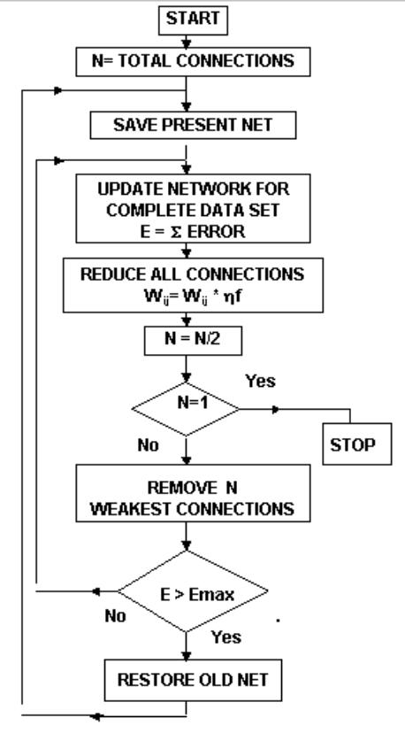
Figure-6
Network optimizing algorithm, where Emax is the maximum tolerable error.
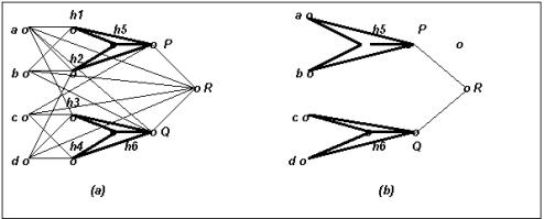
Figure-7
(a) The implantation
of pre-trained XOR Neural Network-
h1, h2, h5, P and h3, h4, h6, Q in a host network. (b) The resultant network
after pruning.
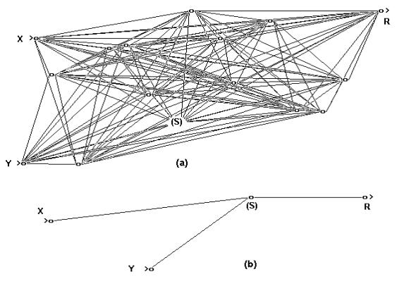
Figure-8 (a)In above example let rad=((X-0.5)2+(Y-
0.5)2)0.5 and if (rad > 0.3) then R=0 else R=1. X and Y
are random analog inputs between 0 to 1. A special neuron S (See text) is
implanted among the hidden neurons in the network. (b) The optimized network,
where all the hidden neurons are eliminated except neuron S.
Experiment-II : Non linear
Boundary Mapping
Problem
In this example, a two dimensional image mapping problem is
studied. A two layer network as shown in figure-8(a)
is configured with two analog inputs, thirteen hidden neurons and a binary
output neuron. Twelve hidden neurons are having conventional exponential sigmoid
type activation function and only one hidden neuron (S)
is used with function of equation
- (7).
Xj = Si
(Wij * Yi2)
and Yj
= 1/(1 +e Xj)
....(7)
The network is first trained to map a circle and then
is pruned. The pruning result is shown
in figure-8(b).
The resultant network has only one hidden neuron and three connections. The only
neuron (S) left in the hidden layer after the pruning operation is the one,
which was specially implanted with the activation function of equation-(7). The final network is also the minimum configuration to
map circular boundary. The inputs and output
of the network of figure- 8(a) and 8(b)
are shown in figure- 9(a), 9(b) and
9(c).
It is shown by the simulation that a feed forward type neural
network can adopt higher order mathematical building blocks during learning
operation. It is shown that such building blocks could use probabilistic pulse
frequency modulated signals using stochastic logic. Such implant has similar
characteristics as biological neurons. Such experiments are very primitive steps
towards direct man machine interface.
(a)
(b)
(c)
Figure-9 (a)
Input training pattern for figure- 8 (a)&(b). (b)Output response of network of
figure- 8(a). (c) Output
response of network of figure-8(b).
[1] Alspector, Allen J., R.B., Hu.V., & Satyanarayana,
S., “ Stochastic learning networks and
their implementation “. In D.Z. Anderson (Ed.), Proceedings of the IEEE
Conference on Neural Information
Processing Systems - Natural and Synthetic, New York: American Institute of
Physics, 1988, pp. 9-21.
[2] Baum Eric. B and Haussler David “ What Size Net Gives
Valid Generalization ?”.Neural Computation, issue of January, 1989.
[3] Karnin E. D, “A simple procedure for pruning
back-propagation trained neural network,” IEEE
Trains. Neural Networks, vol. 1, June, 1990, pp. 239-244.
[4] Lippmann R.P., An introduction to computing with Neural
Nets. IEEE ASSP Magazine, April 1987, pp. 4-22,
[5] Mazumdar Himanshu S, “A mlutilayered feed forward
neural network suitable for VLSI implementation“, Microprocessors and
Microsystems, vol. 19, number 4, May, 1995, pp. 231-234.
[6] Rawal Leena P and Mazumdar Himanshu S,
“ A Neural
Network Tool Box
using C++“,
Computer Society of India, vol. 19, number 2, August 1995, pp. 15-23.
[7] Rumelhart
D.E., Hinton G.E., and Williams R.J.,” Learning Representations by
Back-Propagation Errors”,Nature, Vol.323, No.9, Oct. 1986, pp. 533-536.
Mazumdar Himanshu S.
and Rawal Leena P., "Simulation
of Implant of higher Functions in Randomly Connected Artificial
Neural Network", published in
the Abstracts
proceedings, main papers
XIVA. The International Conference
on Cognitive Systems 1995, Dec. 15th & 16th, New Delhi, Organized by the R
& D Center, NIIT Ltd., INDIA.