|
|
|
| RENT A THINKER |
|
|
|||||
| Home | My Page | Chat | Tik-Tok | ||||
8.1
Abstract
8.2
Introduction
8.3
Back Propagation Algorithm
8.4
Proposed Algorithm
8.5
Hardware Description
8.6
Results
8.7
Appendix
8.8
References
8.9 Publication
A potentially
simplified training strategy for feed forward type neural networks is developed
in view of VLSI implementation. The gradient descent back propagation technique
is simplified to train stochastic type neural hardware. The proposed learning
algorithm uses ADD, SUBTRACT, and LOGICAL operators only. This reduces circuit
complexity with an increase in speed. The Forward and reverse characteristics of
perceptrons are generated using random threshold logic. The supposed hardware
consists of 31 perceptrons per layer working in parallel with a programmable
number of layers working in sequential mode.
Keywords
Stochastic, Multi layer, Neural Network, VLSI
Multilayered
Feed Forward Neural networks have created enormous interest among AI researchers
for their feature extraction capability from input patterns. Their potential as
problem solving tools has also been demonstrated with various learning
algorithms. However, for any serial real world application, such networks should
have a large number of interconnections operating in parallel, obeying
predictable learning rules uniformly throughout the network. The VLSI
implementation of such a network needs a large number of interface lines (pin
connections). Learning algorithms like back propagation need large floating
point operations, which increase rapidly with the increase in number of
perceptrons per layer. It is thus necessary to give adequate stress to the
simplification of the learning algorithm so as to reduce the computational need
for massive parallelism.
This paper describes a simplified technique to implement multi layered
Neural network using random number generators. The gradient descent technique is
modified to implement stochastic logic. The prototype network built by us
consists of maximum of 31 perceptrons in each layer. The learning algorithms
uses only ADD and SUBTRACT and LOGICAL operations. Interlayer communication
needs only one bit per output and hence minimizes the data path considerably.
We first
review briefly the back propagation technique, which is normally used for
training feed forward type neural networks. The input-output characteristic
function of perceptrons is chosen such that it is continuous and its derivative
is bounded between definite limits for a large dynamic range of input.
Consider
a three layer network of units Yi, Yj and Yk
interconnected through weights Wji and Wkj such that
Xj
= Si Wji * Yi;
Yi = f(Xj)
and
Xk = Sj Wkj * Yj;
Yj = f(Xk)
(First Layer)
(Second Layer)
where Y
= F(X) represents the input-output characteristic function of the perceptrons,
which is usually chosen to be of the form:
f(x) = 1 / (1 + e –x ).
The
weights Wji and Wkj are modified using the BP algorithm as
follows.
Wkj
= Wkj + n * Y * [(Yk – Dk) * Yk *
(1 – Yk)}]
(1)
Wkj
= Wkj + n * Yj * {Yj * (1 – Yj)}
* Skk [(Yk – Dk)
* {Yk * (1 – Yk)} * Wkj]
(2)
Where n
is a constant less than 1 and Dk is the desired output. Most of the
operators in equations (1) and (2) operate on real variables. Hence it is
difficult to implement a large number of perceptrons working in parallel in a
VLSI.
It has
been shown that the choice of the perceptron’s characteristics is not very
critical for convergence of error during training. This paper suggests one such
choice which reduces the computational requirement drastically without affecting
the error convergence property during training.
We will analyze
the significance of each factor in expressions (1) and (2) in order to replace
them by suitable probability functions.
(Yk
– Dk) is the departure of output Yk from the desired
value Dk. Yk * (1 – Yk) is the measure of
willingness of the Kth output perceptron to learn. This is measured by its
nearness from its average value (0.5). This factor plays an important role in
training. Wkj is the back propagation signal path’s conductance. Yj
* (1 – Yj) is similar to the above term Yk * (1 – Yk)
for a hidden layer perceptron. Yi is the excitation potential for the
network.
In this
architecture, we have considered all the perceptrons Yi, Yj
and Yk having binary output. In the proposed system the
perceptron’s forward pass transfer characteristics are generated by a
threshold detector having a random bias value as shown in Figure 1. This is
equivalent to a choice of input-output characteristic function Y = f(X) of the
form
Y = 1 for (X + r) > 0
= 0 for (X + r)
£
0
(3)
where r is a
random integer inside the dynamic range of X. Yj and Yk
are calculated using the above expression in the forward pass. This has two
advantages: the value of Yj is binary but is statistically continuous
in the dynamic range of learning and the computation of Xk (for the
next layer) does not need any multiplications.
In the backward pass, a term of the form Yk * (1 – Yk)
is desirable. This term increases the sensitivity of Wkj near the
threshold value of Xk. Equivalently; the network’s willingness to
learn or forget is inversely proportional to the distance of Xj from
the threshold. Considering this, a simplified reverse characteristic function
R(X) as shown in figure is used to replace the terms of the form Yk *
(1 – Yk) in equations (1) and (2).
R(X) = 0 for abs (X) > r
= 1 for abs (X) £
r
(4)
where r is a
random integer in the range 0 £
r < N and the dynamic range of X for learning is (-N to +N).
|
|
|
Figure
1: The forward and reverse characteristics of the proposed stochastic
function along with the exponential sigmoid function (solid line).
The value of N
is dependent on the network configuration. To improve the dynamic range of
inputs and the rate of convergence the following options are listed.
·
Use of N as random
integer itself;
·
Use of r as a weighted
random number;
·
Adjusting the value of N
gradually as the error converges.
Figure 2 shows
a simplified hardware diagram of the multi-layered neuroengine. The system
consists of three 32 bit registers, one 16 bit adder and a random number
generator which are connected to memory via a 16 bit bus. A PROM based sequence
controller generates all necessary control signals for different passes and is
also used to store the configuration of the network.
Register SH1 is loaded with input Yi, which is rotated 32
times using 1024 clock cycles. In every clock cycle let the corresponding weight
Wji is fetched from external RAM and depending on the MSB of SH1, Wji
is added to or subtracted from the contents of the latch. After one complete
cycle of SH1 Xj is computed in LCH. In training mode a random number
is added to Xj through BF3. The sign bit of Xj represents Yj which is stored in
SH3. All Yj are computed from Wji and Yj in 1024 clock cycles.
The learning
mode needs five passes for a two-layer network as follows.
1.
Compute Yi
2.
Compute Yk
3.
Correct Wkj
4.
Compute Dj
5.
Correct Wji
The complete
two layer learn cycle needs about 7000 clock cycles, which less than one
millisecond.
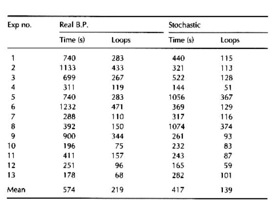
The above
algorithm is first tested in a simulated environment using 16bit integer
arithmetic. The results are compared with those from the original back
propagation algorithm using real number arithmetic. An IBM-386 computer with
co-processor was used for testing both the methods. Both the networks were
configured with eight input units, eight hidden units, and one output unit. All
parameters in both types of networks were optimized for minimum convergence
time. The output function was chosen as mirror symmetry detection of input data.
The convergence success rate was found to be larger and convergence time shorter
in the proposed algorithm as compared to the BP algorithm. Some sample results
are shown in table 1. TTL based hardware has also been tested for successful
convergence for various output functions.
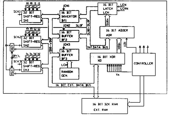
Figure 2:
Block diagram of the proposed multi layered feed forward neural network.
Table 1:
Sample Results.
A sample
program for three-layer network, N0, N1, N² and N³ are constants adjusted for
dynamic range and rate of convergence.
PROCEDURE forward_pass;
BEGIN
FOR
j:=0 TO jmax DO
BEGIN
xj[j]:=0;
FOR i:=0 TO imax+1 DO
IF yi[i]>0 THEN xj[j]:=
xj[j] + wji[j,i];
IF xj[j]>random(N0)
THEN yj[j]:=1 ELSE yj[j]:=0;
END;
FOR
k:=0 TO kmax DO
BEGIN
xk[k]:=0;
FOR j:=0 TO jmax+1 DO
IF yj[j]>0 THEN xk[k] := xk[k] + wkj[k,j];
IF xk[k]>random(N0) THEN
yk[k]:=1 ELSE
yk[k]:=0;
END;
END;
PROCEDURE training_pass;
BEGIN
FOR j:=0 TO jmax+1 DO outj[j]:=0;
FOR k:=0 TO kmax DO
BEGIN
IF abs(xk[k]) > random(N1) THEN p:=0 ELSE p:=1;
d:=out[k]-yk[k];
IF d<>0 THEN
FOR j:=0 TO jmax+1 DO
BEGIN
IF yj[j]>0 THEN wkj[k,j] := wkj[k,j] +d
ELSE wkj[k,j] := wkj[k,j] -d;
IF p>0 THEN
IF d>0 THEN outj[j]:=outj[j] + wkj[k,j]
ELSE outj[j]:=outj[j] - wkj[k,j];
END;
END;
FOR j:=0 TO jmax DO
BEGIN
IF abs(xj[j]) > random(N2) THEN a:=0 ELSE a:=1;
IF abs(outj[j]) > random(N3) THEN b:=1 ELSE b:=0;
d:=a and b;
IF d<>0 THEN
IF outj[j]>0 THEN
FOR i:=0 TO imax+1 DO
IF yi[i]>0 THEN
wji[j,i] := wji[j,i] +d
ELSE wji[j,i] := wji[j,i] -d
ELSE
FOR i:=0 TO imax+1 DO
IF yi[i]>0 THEN wji[j,i] := wji[j,i] -d
ELSE
wji[j,i] := wji[j,i] +d;
END;
END;
[1] Rumelhart
D.E., Hinton G.E., and Williams R.J., Learning Representations by
Back-Propagation Errors. Nature, Vol.323, No. 9, pp.533-536, Oct.1986.
[2] David S.
Touretzky and Dean A. Pomerleau, "What's Hidden in the Hidden
Layers?", BYTE, pp.227-233, August 1989.
[3] Widrow B.,
Winter R.G., and Baxter R.A., (1988). Layered Neural Nets for Pattern
Recognition, Transactions on Acoustics, Speech and Signal Processing, vol. 36
No. 7 July 1988.
[4]
Lang,K.J., Waibel,A.H., and
Hinton G.E., A Time-Delay Neural
Network Architecture for Isolated Word Recognition. Neural Networks, Vol.3,
pp.23-43, 1990.
[5]
Alspector, J.Allen, R.B.,Hu.V., & Satyanarayana, S., Stochastic learning
networks and their implementation. In D.Z. Anderson (Ed.), Proceedings of the
IEEE Conference on Neural Information Processing Systems - Natural and
Synthetic, pp.9-21, New York American Institute of Physics, 1988.
[6] Gagan
MirchandanI and WeI Cao, "On Hidden Nodes for Neural Net", IEEE
Transactions on Circuits and Systems Vol.36, No.µ May 1989.
[7] Lippmann
R.P., An introduction to computing with Neural Nets. IEEE ASSÐ Magazine, pð
4-22, April,1987.
[8] W P. Jones
and Josiah Hoskins, "Back-Propagation” BYTE, pp.155-162, October 1987.
Himanshu S. Mazumdar, " A VLSI implementation of multilayered feed forward neural network ", published in the international journal -Microprocessors and Microsystems, vol.- 19, number-4, May, pp.231-235, USA, 1995.